
Follow the transformation
Represent inputs/parameters as vectors or matrices.
Compute the model score/prediction.
Evaluate a loss against the observed target.
Gradient Descent supplies mathematical intuition for how models represent predictions and learn from error.
Gradient Descent supplies mathematical intuition for how models represent predictions and learn from error. Vectors encode features/parameters, dot products create linear scores, loss functions quantify disagreement with targets, and gradients point toward local directions of change in differentiable objectives.
Gradient Descent matters because model predictions and optimisation are expressed through vectors, linear algebra, probability and loss functions. Connecting the mathematics to a concrete prediction or parameter update makes later algorithms much easier to understand.
Treat this as a sequence of observable decisions rather than one opaque command. Stage 1: Represent inputs/parameters as vectors or matrices. Stage 2: Compute the model score/prediction. Stage 3: Evaluate a loss against the observed target. Final checkpoint: Update parameters in a direction that reduces the objective, balancing fit and generalisation.
Represent inputs/parameters as vectors or matrices.
Compute the model score/prediction.
Evaluate a loss against the observed target.
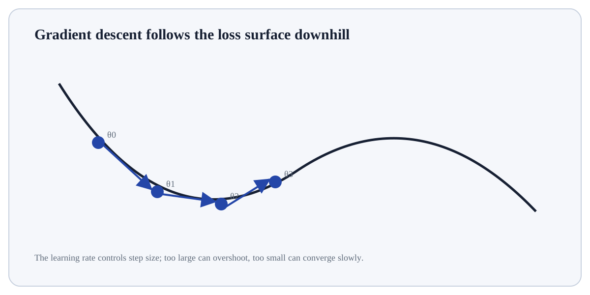
Represent inputs/parameters as vectors or matrices. For Gradient Descent, identify the exact state before this stage, the operation or rule applied here, and the observable state afterwards so the mechanism remains inspectable.
# Step 1 — Compute the right-hand expression and store its result in `theta` for the next step.
theta=0.0
# Step 2 — Compute the right-hand expression and store its result in `learning_rate` for the next step.
learning_rate=0.1
# L=(theta-3)^2 => gradient=2(theta-3)
# Step 3 — Iterate through the collection so the indented block is applied once for each item.
for step in range(5):
    # Step 4 — Compute the right-hand expression and store its result in `grad` for the next step.
    grad=2*(theta-3)
    # Step 5 — Execute this statement and inspect how it changes the current value, object or program state.
    theta -= learning_rate*grad
    # Step 6 — Display the current value explicitly so the result/state can be inspected during execution.
print(step+1, round(theta,3))theta moves 0 → 0.6 → 1.08 → 1.464 → ... toward the minimum at 3.
For Gradient Descent, connect the displayed result to the specific input and mechanism above; independently verify one value/state change rather than treating successful execution as proof.
LossObjective contribution for prediction error.GradientVector of partial derivatives of loss with respect to parameters.Learning rateStep-size hyperparameter for gradient updates.BiasSystematic error from restrictive assumptions.VarianceSensitivity of the fitted model to training-sample variation.Use Gradient Descent when the mathematical object directly represents the model quantity or transformation being reasoned about and dimensions/units are explicit.
Stop if vectors/matrices, dimensions, signs, scales or probability assumptions are not defined; symbolic manipulation without those definitions can produce a formally valid but meaningless result.
Build a tiny, inspectable example of Gradient Descent. First represent inputs/parameters as vectors or matrices. Then compute the model score/prediction. Write the expected result before running it, and explain one condition that would make the result misleading or invalid.
Before trusting a result from Gradient Descent, which check provides the strongest evidence that you understand and applied it correctly?
Step 1Represent inputs/parameters as vectors or matrices.Step 2Compute the model score/prediction.Step 3Evaluate a loss against the observed target.Step 4Compute or approximate how the loss changes with parameters.