
Follow the transformation
Standardise features first when different measurement scales should contribute comparably.
Centre the training data.
Compute covariance structure (or use SVD) and obtain orthogonal component directions.
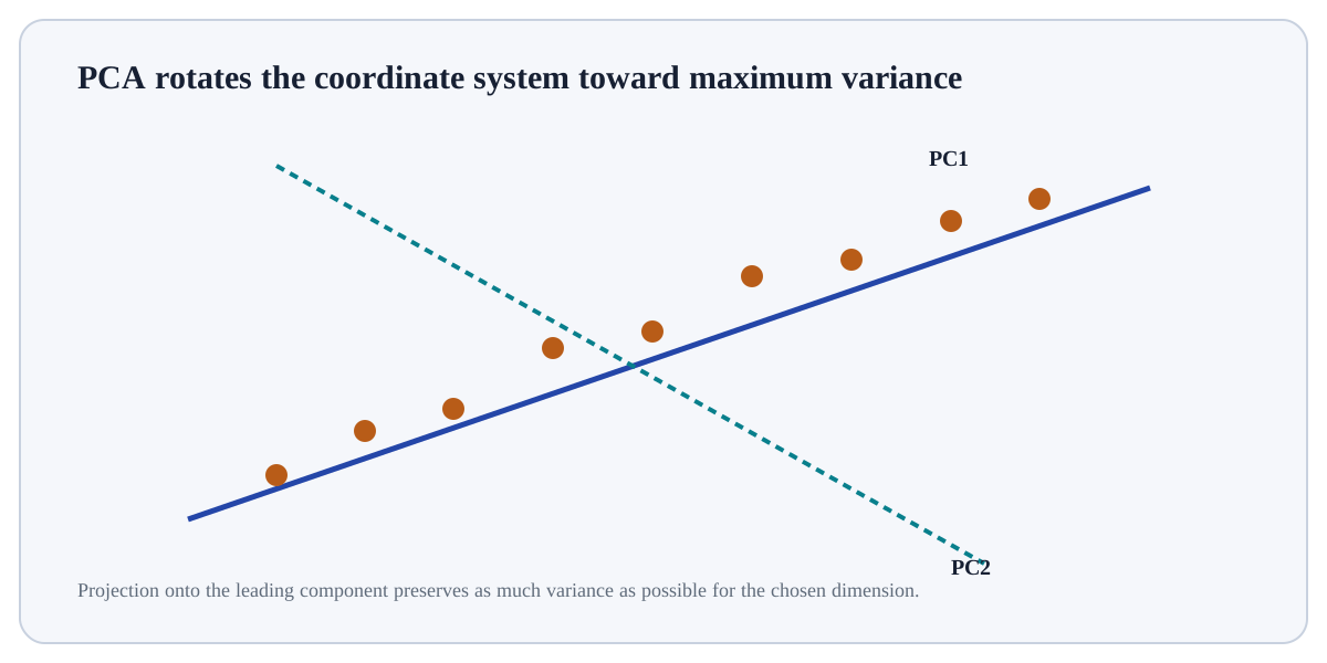
Principal Component Analysis (PCA) is an unsupervised linear transformation that rotates centred data into orthogonal directions of decreasing variance.
Principal Component Analysis (PCA) is an unsupervised linear transformation that rotates centred data into orthogonal directions of decreasing variance. Each principal component is a weighted linear combination of the original features; projecting onto the first components can compress correlated data while preserving as much variance as possible under a linear criterion.
PCA matters because unsupervised methods impose a particular notion of structure—variance, distance, density or probability—without target labels. The discovered representation or clusters must therefore be interpreted relative to that chosen notion.
Treat this as a sequence of observable decisions rather than one opaque command. Stage 1: Standardise features first when different measurement scales should contribute comparably. Stage 2: Centre the training data. Stage 3: Compute covariance structure (or use SVD) and obtain orthogonal component directions. Final checkpoint: Interpret loadings and reconstruction/variance trade-offs; fit PCA inside cross-validation.
Standardise features first when different measurement scales should contribute comparably.
Centre the training data.
Compute covariance structure (or use SVD) and obtain orthogonal component directions.
Standardise features first when different measurement scales should contribute comparably. For PCA, identify the exact state before this stage, the operation or rule applied here, and the observable state afterwards so the mechanism remains inspectable.
# Step 1 — Import the module so its functions/classes are available to the rest of this example.
import numpy as np
# Step 2 — Import only the named objects needed by the following steps, keeping dependencies explicit.
from sklearn.decomposition import PCA
# Step 3 — Import only the named objects needed by the following steps, keeping dependencies explicit.
from sklearn.preprocessing import StandardScaler
# Step 4 — Construct `X` as an array so vectorised numerical operations can be applied consistently.
X = np.array([[1,10],[2,20],[3,31],[4,39],[5,51]], dtype=float)
# Step 5 — Fit the transformation on the training input and immediately transform that same input.
Xs = StandardScaler().fit_transform(X)
# Step 6 — Fit the model or transformer, learning its parameters from the supplied training data.
pca = PCA(n_components=1).fit(Xs)
# Step 7 — Apply the already-fitted transformation without relearning its parameters from this data.
Z = pca.transform(Xs)
# Step 8 — Display the current value explicitly so the result/state can be inspected during execution.
print("explained variance ratio:", np.round(pca.explained_variance_ratio_, 3))
# Step 9 — Display the current value explicitly so the result/state can be inspected during execution.
print("scores shape:", Z.shape)explained variance ratio: [about 0.999] scores shape: (5, 1)
For PCA, connect the displayed result to the specific input and mechanism above; independently verify one value/state change rather than treating successful execution as proof.
Feature constructionCreate new variables such as ratios, interactions or lags.Feature selectionKeep a subset of original/constructed variables.PCACreate orthogonal linear combinations ordered by explained variance.TF-IDFRepresent text by term importance relative to document frequency.Use PCA when the goal is to discover or represent structure without a supervised target and the chosen similarity/density/latent assumptions match the data.
Reconsider the method when feature scaling, distance choice, cluster shape, density variation or embedding purpose makes the discovered structure unstable or uninterpretable.
Build a tiny, inspectable example of PCA. First standardise features first when different measurement scales should contribute comparably. Then centre the training data. Write the expected result before running it, and explain one condition that would make the result misleading or invalid.
Before trusting a result from PCA, which check provides the strongest evidence that you understand and applied it correctly?
Step 1Standardise features first when different measurement scales should contribute comparably.Step 2Centre the training data.Step 3Compute covariance structure (or use SVD) and obtain orthogonal component directions.Step 4Order components by explained variance.