
Follow the transformation
Construct the design matrix X and target y.
Estimate coefficients β that minimise squared residuals.
Generate predictions ŷ = Xβ (plus intercept).
Linear regression models a continuous target as a weighted sum of input features plus an intercept.
Linear regression models a continuous target as a weighted sum of input features plus an intercept. Ordinary least squares chooses coefficients that minimise the sum of squared residuals between observed and predicted targets.
Linear Regression matters because linear models provide an interpretable baseline and expose central ideas such as coefficient estimation, probability links and regularisation. They also show clearly how preprocessing and penalty choices affect fitted parameters.
Treat this as a sequence of observable decisions rather than one opaque command. Stage 1: Construct the design matrix X and target y. Stage 2: Estimate coefficients β that minimise squared residuals. Stage 3: Generate predictions ŷ = Xβ (plus intercept). Final checkpoint: Use validation to assess predictive generalisation; regularise when complexity/collinearity warrants it.
Construct the design matrix X and target y.
Estimate coefficients β that minimise squared residuals.
Generate predictions ŷ = Xβ (plus intercept).
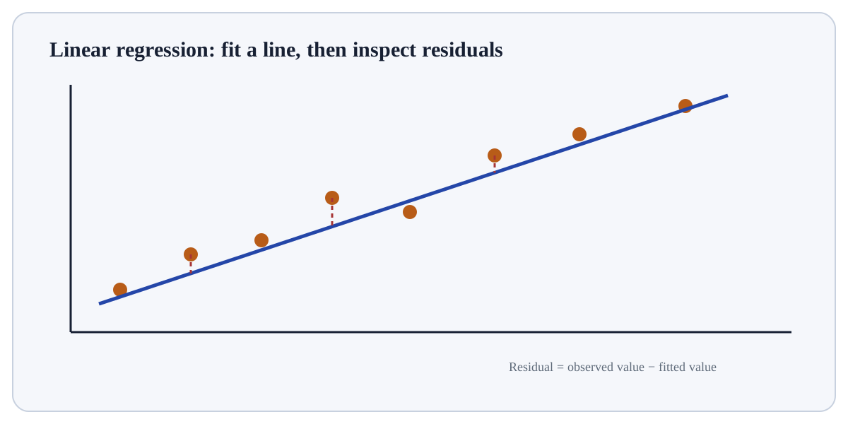
Construct the design matrix X and target y. This is an input-preparation stage for Linear Regression. Verify the relevant type, shape, units, keys, missingness or assumptions before later steps depend on them.
# Step 1 — Import the module so its functions/classes are available to the rest of this example.
import numpy as np
# Step 2 — Import only the named objects needed by the following steps, keeping dependencies explicit.
from sklearn.linear_model import LinearRegression
# Step 3 — Construct `X` as an array so vectorised numerical operations can be applied consistently.
X=np.array([[1],[2],[3],[4]],float); y=np.array([2,4.2,5.8,8.1])
# Step 4 — Fit the model or transformer, learning its parameters from the supplied training data.
m=LinearRegression().fit(X,y)
# Step 5 — Display the current value explicitly so the result/state can be inspected during execution.
print(round(m.coef_[0],2), round(m.intercept_,2))
# Step 6 — Display the current value explicitly so the result/state can be inspected during execution.
print(round(m.predict([[5]])[0],2))A slope near 2 and prediction near 10 illustrate fitting a linear relationship by squared-error minimisation.
For Linear Regression, connect the reported result to the exact training/validation/prediction step that produced it and check one prediction, fold or metric component independently.
Linear regressionContinuous target; linear in chosen features.RidgeLinear regression with L2 shrinkage.LassoLinear regression with L1 shrinkage and possible sparsity.Polynomial featuresStill a linear model in transformed features, but nonlinear in the original input.Use Linear Regression when its inductive assumptions fit the feature/target structure and it can be compared fairly with a simpler baseline on unseen data.
Prefer a simpler or different model when the sample size, representation, computational budget, interpretability requirement or data geometry conflicts with this method.
Build a tiny, inspectable example of Linear Regression. First construct the design matrix X and target y. Then estimate coefficients β that minimise squared residuals. Write the expected result before running it, and explain one condition that would make the result misleading or invalid.
Before trusting a result from Linear Regression, which check provides the strongest evidence that you understand and applied it correctly?
Step 1Construct the design matrix X and target y.Step 2Estimate coefficients β that minimise squared residuals.Step 3Generate predictions ŷ = Xβ (plus intercept).Step 4Inspect residuals for nonlinearity, heteroscedasticity, outliers and dependence.