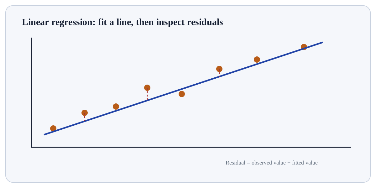
Linear regression learns coefficients that make predicted values close to observed targets under a squared-error objective. Coefficients quantify conditional linear associations.
Building interactive view…
Understand
Build the mental model
Linear regression learns coefficients that make predicted values close to observed targets under a squared-error objective. Coefficients quantify conditional linear associations. Inspect residuals, nonlinearity, influential points and extrapolation. Coefficients are not automatically causal effects.
Click a stage to inspect what happens, what changes, and what should be checked before moving on.
Stage 1
Features
Identify exactly what enters this stage: its shape, type, scale, units and any missing or invalid values that could alter the next operation. Technical context for Linear Regression: OLS minimises the sum of squared residuals. Matrix form gives β̂=(XᵀX)⁻¹Xᵀy when conditions permit; regularised variants change the objective to stabilise estimates.
Practitioner checkpoint: Inspect residuals, nonlinearity, influential points and extrapolation. Coefficients are not automatically causal effects.
What happens if…?
Break the assumption deliberately
Add one extreme outlier and watch squared error pull the fitted line toward it.
Move the control and explain what you expect before reading the visual.
Technical lens
Formalise what the visual is doing
OLS minimises the sum of squared residuals. Matrix form gives β̂=(XᵀX)⁻¹Xᵀy when conditions permit; regularised variants change the objective to stabilise estimates.
Technical questionUse a tiny case to make the mechanism observable. OLS minimises the sum of squared residuals. Matrix form gives β̂=(XᵀX)⁻¹Xᵀy when conditions permit; regularised variants change the objective to stabilise estimates. Verify one intermediate quantity, state change or mapping independently; then predict the consequence of this change: Add one extreme outlier and watch squared error pull the fitted line toward it.
Practitioner lens
Use it responsibly
Inspect residuals, nonlinearity, influential points and extrapolation. Coefficients are not automatically causal effects.
Transfer testAssuming linearity in the raw input when transformed features may be needed.
Worked exploration
Use the visual as an experiment, not decoration
Fit points near y = 2x + 1. Draw residuals vertically from points to the line. Square each residual and add them; move the line slightly and observe how the total squared error changes.
Technical lens
OLS minimises the sum of squared residuals. Matrix form gives β̂=(XᵀX)⁻¹Xᵀy when conditions permit; regularised variants change the objective to stabilise estimates.
Practitioner check
Inspect residuals, nonlinearity, influential points and extrapolation. Coefficients are not automatically causal effects.
Prediction before interaction
Add one extreme outlier and watch squared error pull the fitted line toward it.
Exploration walkthrough
Turn the interaction into an evidence trail
Fit points near y = 2x + 1. Draw residuals vertically from points to the line. Square each residual and add them; move the line slightly and observe how the total squared error changes. Before moving the control, state your prediction. After the visual changes, name the specific state, statistic, boundary or mapping that changed and explain why that change is consistent—or inconsistent—with your prediction.
Record one observable quantity before the interaction and the same quantity afterwards.
Change one factor at a time so the causal effect of the control is inspectable.
Use an edge or failure case to discover where the concept stops behaving as the simple story suggests.
Static orientation diagram for Linear Regression; use the interactive visual above to test how the relationships change.
Reference depth
Open the complete material
The flagship experience is the map. These pages contain the roads.