How does a linear model become a probability classifier?
Start here
How does a linear model become a probability classifier?
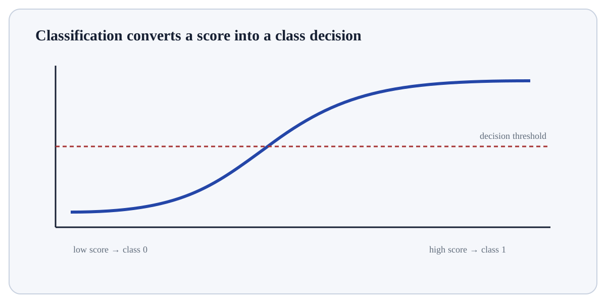
Logistic regression learns a linear score and maps it through the logistic function, producing a probability that can be thresholded into a class decision.
Building interactive view…
Understand
Build the mental model
Logistic regression learns a linear score and maps it through the logistic function, producing a probability that can be thresholded into a class decision. Use it as a strong interpretable baseline. Check calibration, class imbalance, multicollinearity and nonlinear patterns.
Click a stage to inspect what happens, what changes, and what should be checked before moving on.
Stage 1
Linear score
Quantify the discrepancy here rather than relying on visual impression alone. The value should connect directly to the objective or diagnostic being optimised or inspected. Technical context for Logistic Regression: The model is linear in log-odds. Training minimises log loss; regularisation controls coefficient magnitude. The decision boundary is linear unless features are transformed.
Practitioner checkpoint: Use it as a strong interpretable baseline. Check calibration, class imbalance, multicollinearity and nonlinear patterns.
What happens if…?
Break the assumption deliberately
Move the classification threshold without retraining and watch precision/recall trade places.
Move the control and explain what you expect before reading the visual.
Technical lens
Formalise what the visual is doing
The model is linear in log-odds. Training minimises log loss; regularisation controls coefficient magnitude. The decision boundary is linear unless features are transformed.
Technical questionUse a tiny case to make the mechanism observable. The model is linear in log-odds. Training minimises log loss; regularisation controls coefficient magnitude. The decision boundary is linear unless features are transformed. Verify one intermediate quantity, state change or mapping independently; then predict the consequence of this change: Move the classification threshold without retraining and watch precision/recall trade places.
Practitioner lens
Use it responsibly
Use it as a strong interpretable baseline. Check calibration, class imbalance, multicollinearity and nonlinear patterns.
Transfer testCalling the 0.5 threshold universally optimal.
Worked exploration
Use the visual as an experiment, not decoration
Compute a linear score for two cases, pass each through the sigmoid to obtain probabilities, then apply thresholds 0.5 and 0.8. The probabilities stay fixed while class decisions change.
Technical lens
The model is linear in log-odds. Training minimises log loss; regularisation controls coefficient magnitude. The decision boundary is linear unless features are transformed.
Practitioner check
Use it as a strong interpretable baseline. Check calibration, class imbalance, multicollinearity and nonlinear patterns.
Prediction before interaction
Move the classification threshold without retraining and watch precision/recall trade places.
Exploration walkthrough
Turn the interaction into an evidence trail
Compute a linear score for two cases, pass each through the sigmoid to obtain probabilities, then apply thresholds 0.5 and 0.8. The probabilities stay fixed while class decisions change. Before moving the control, state your prediction. After the visual changes, name the specific state, statistic, boundary or mapping that changed and explain why that change is consistent—or inconsistent—with your prediction.
Record one observable quantity before the interaction and the same quantity afterwards.
Change one factor at a time so the causal effect of the control is inspectable.
Use an edge or failure case to discover where the concept stops behaving as the simple story suggests.
Static orientation diagram for Logistic Regression; use the interactive visual above to test how the relationships change.
Reference depth
Open the complete material
The flagship experience is the map. These pages contain the roads.